Useful QS
What is a Lagrangian and what is the Hamiltonian? How are they related?↩
The energy-momentum tensor \(T^\mu_\nu:=j^\mu_\nu=\partial_\nu\phi\frac{\partial \mathcal{L}}{\partial(\partial_mu \phi)}-\eta^\mu_\nu \mathcal{L} ~\text{and}~ \partial_\mu T^{\mu\nu}\)(Not symmetric)
Relation: \(P^0=\int d^3x T^{00}=\int d^3x \mathcal{H}=H\)
with canonical momenta: \(\mathcal{H}=\pi\partial_0\phi -\mathcal{L}\)
What are the canonical momenta?↩
\(\pi=\frac{\partial\mathcal{L}}{\partial(\partial_0 \phi)}\)(in real scalar field \(\partial_0 \phi(\mathbf{x})\)) The commutation relation is: \([\phi(\mathbf{x}),\pi(\mathbf{y})]=\mathrm{i}\delta(\mathbf{x-y})\qquad[\phi(\mathbf{x}),\phi(\mathbf{y})]=[\pi(\mathbf{x}),\pi(\mathbf{y})]=0\)
| scalar | complex scalar | spinor | gauge | QED | |
|---|---|---|---|---|---|
| \(\mathcal{L}\) | \(\partial_\mu \phi \partial^\mu \phi-m^2 \phi^2\) | \(\partial_\mu \phi \partial^\mu \phi^*-m^2 \phi \phi^*\) | \(\bar{\psi}(\mathrm{i} \cancel{\partial}-m) \psi\) | \(-\frac{1}{4} F_{\mu v} F^{\mu v}\) | \(-\frac{1}{2} \operatorname{tr}_f F_{\mu \nu} F^{\mu v}+\bar{\psi}(\mathrm{i} \cancel{D}-m) \psi\) |
| EoM | \(\left(\partial^2+m^2\right) \phi(x)=0\) | - | \(\begin{aligned} \mathrm{i} \bar{\sigma}^\mu \partial_\mu \psi_L=0 \\ \mathrm{i} \sigma^\mu \partial_\mu \psi_R=0\end{aligned}\) | \(\partial_\rho \partial^\rho A^v=0\) | - |
How are scalar/spinor/gauge fields quantised?↩
- Scalar field
- Normal field OP \(\begin{aligned} \phi(x) & =\int \frac{\mathrm{d}^3 p}{(2 \pi)^3} \frac{1}{\sqrt{2 \omega_{\mathbf{p}}}}\left(a(\boldsymbol{p}) e^{-\mathrm{i} p x}+a^{\dagger}(\boldsymbol{p}) e^{\mathrm{i} p x}\right) \\ \pi(x) & =-\mathrm{i} \int \frac{\mathrm{d}^3 p}{(2 \pi)^3} \sqrt{\frac{\omega_{\mathbf{p}}}{2}}\left(a(\boldsymbol{p}) e^{-\mathrm{i} p x}-a^{\dagger}(\boldsymbol{p}) e^{\mathrm{i} p x}\right)\end{aligned}\)
- Fourier Transformed OP \(\begin{aligned} & \tilde{\phi}(\boldsymbol{p})=\int \mathrm{d}^3 x e^{-\mathrm{i} \boldsymbol{p} x} \phi(\boldsymbol{x})=\frac{1}{\sqrt{2 \omega_{\boldsymbol{p}}}}\left(a(\boldsymbol{p})+a^{\dagger}(-\boldsymbol{p})\right) \\ & \tilde{\pi}(\boldsymbol{p})=\int \mathrm{d}^3 x e^{-\mathrm{i} \boldsymbol{p} x} \partial^0 \phi(\boldsymbol{x})=-i \sqrt{\frac{\omega_{\mathbf{p}}}{2}}\left(a(\boldsymbol{p})-a^{\dagger}(-\boldsymbol{p})\right)\end{aligned}\)
- Creation and annihilation operators \(\begin{aligned} a(\boldsymbol{p}) & =\sqrt{\frac{\omega_{\mathbf{p}}}{2}} \tilde{\phi}(\boldsymbol{p})+\mathrm{i} \frac{1}{\sqrt{2 \omega_{\mathbf{p}}}} \tilde{\pi}(\boldsymbol{p}) \\ a^{\dagger}(-\boldsymbol{p}) & =\sqrt{\frac{\omega_{\mathbf{p}}}{2}} \tilde{\phi}(\boldsymbol{p})-\mathrm{i} \frac{1}{\sqrt{2 \omega_{\mathbf{p}}}} \tilde{\pi}(\boldsymbol{p}) .\end{aligned}\)
- Hamiltonian \(H=\int \frac{\mathrm{d}^3 p}{(2 \pi)^3} \frac{1}{2}\left[\tilde{\pi}(\boldsymbol{p}) \tilde{\pi}(-\boldsymbol{p})+\omega_{\mathbf{p}}^2 \tilde{\phi}(\boldsymbol{p}) \tilde{\phi}(-\boldsymbol{p})\right]=\int \frac{\mathrm{d}^3 p}{(2 \pi)^3} \omega_{\mathbf{p}} a^{\dagger}(\boldsymbol{p}) a(\boldsymbol{p})\)
-
Relation
- \(\begin{aligned} & {[\phi(t, \boldsymbol{x}), \pi(t, \mathbf{y})]=\mathrm{i} \delta(\boldsymbol{x}-\mathbf{y})} \\ & {[\phi(t, \boldsymbol{x}), \phi(t, \mathbf{y})]=0=[\pi(t, \boldsymbol{x}), \pi(t, \mathbf{y})]}\end{aligned}\)
- \(\begin{aligned} & [\tilde{\phi}(\boldsymbol{p}), \tilde{\pi}(\mathbf{q})] =\mathrm{i}(2 \pi)^3 \delta(\boldsymbol{p}+\mathbf{q}) \\ & [\tilde{\phi}(\boldsymbol{p}), \tilde{\phi}(\mathbf{q})]=0=[\tilde{\pi}(\boldsymbol{p}), \tilde{\pi}(\mathbf{q})]\end{aligned}\)
- \(\begin{aligned} &[a(\boldsymbol{p}), a^{\dagger}(\mathbf{q})]=(2 \pi)^3 \delta(\boldsymbol{p}-\mathbf{q}) \\ & [a(\boldsymbol{p}), a(\mathbf{q})]=0=\left[a^{\dagger}(\boldsymbol{p}), a^{\dagger}(\mathbf{q})\right]\end{aligned}\)
-
Complex Scalar field
- Fourier Transformed OP \(\begin{aligned} & \phi(\mathbf{x})=\int \frac{\mathrm{d}^3 p}{(2 \pi)^3} \frac{1}{\sqrt{2 \omega_{\mathbf{p}}}}\left(a(\boldsymbol{p}) e^{\mathrm{i} \mathbf{p x}}+b^{\dagger}(\boldsymbol{p}) e^{-\mathrm{i} \mathbf{p x}}\right) \\ & \pi(\mathbf{x})=\partial^0 \phi^{\dagger}(x)=-\mathrm{i} \int \frac{\mathrm{d}^3 p}{(2 \pi)^3} \sqrt{\frac{\omega_{\mathbf{p}}}{2}}\left(b(\boldsymbol{p}) e^{\mathrm{i} \mathbf{p x}}-a^{\dagger}(\boldsymbol{p}) e^{-\mathrm{i} \mathbf{p x}}\right)\end{aligned}\) with \(a=\frac{1}{\sqrt{2}}\left(a_1+\mathrm{i} a_2\right), \quad b=\frac{1}{\sqrt{2}}\left(a_1-\mathrm{i} a_2\right)\)
-
Hamiltonian \(H=\frac{1}{2} \int \frac{\mathrm{d}^3 p}{(2 \pi)^3}\left[\tilde{\pi}(\boldsymbol{p}) \tilde{\pi}^{\dagger}(\boldsymbol{p})+\omega_{\mathbf{p}}^2 \tilde{\phi}(\boldsymbol{p}) \tilde{\phi}^{\dagger}(\boldsymbol{p})\right]=\frac{1}{2} \int \frac{\mathrm{d}^3 p}{(2 \pi)^3} \omega_{\mathbf{p}}\left[a^{\dagger}(\boldsymbol{p}) a(\boldsymbol{p})+b^{\dagger}(\boldsymbol{p}) b(\boldsymbol{p})\right]\)
- Relation
- \(\begin{aligned} &{[\phi(\boldsymbol{x}), \pi(\mathbf{y})] } =\mathrm{i} \delta(\boldsymbol{x}-\mathbf{y}) \\& {\left[a(\boldsymbol{p}), a^{\dagger}(\boldsymbol{q})\right] } =(2 \pi)^3 \delta(\boldsymbol{p}-\boldsymbol{q}) \\ &{\left[b(\boldsymbol{p}), b^{\dagger}(\boldsymbol{q})\right] } =(2 \pi)^3 \delta(\boldsymbol{p}-\boldsymbol{q})\end{aligned}\)
-
Spinor field
- Fourier Transformed OP \(\psi(x)=\int \frac{\mathrm{d}^3 p}{(2 \pi)^3} \frac{1}{\sqrt{2 p^0}} \sum_s\left[e^{-\mathrm{i} p x} a_s(\boldsymbol{p}) u_s(\boldsymbol{p})+e^{+\mathrm{i} p x} b_s^{\dagger}(\boldsymbol{p}) v_s(\boldsymbol{p})\right]\)
-
Hamiltonian \(H =\int \mathrm{d}^3 x \psi^{\dagger}(\mathbf{x}) \gamma^0(\mathrm{i} \boldsymbol{\gamma} \boldsymbol{\partial}+m) \psi(\boldsymbol{x}) =\int \frac{\mathrm{d}^3 p}{(2 \pi)^3} \frac{2 p^0}{2 p^0} p^0 \sum_s\left[a_s^{\dagger}(\boldsymbol{p}) a_s(\boldsymbol{p})-b_s(\boldsymbol{p}) b_s^{\dagger}(\boldsymbol{p})\right]\)
- Relation(mainly anti-commutation)
- \(\begin{aligned} & \left\{a_s(\boldsymbol{p}), a_r^{\dagger}(\boldsymbol{q})\right\}=(2 \pi)^3 \delta_{s r} \delta(\boldsymbol{p}-\boldsymbol{q}) \\ & \left\{b_s(\boldsymbol{p}), b_r^{\dagger}(\boldsymbol{q})\right\}=(2 \pi)^3 \delta_{s r} \delta(\boldsymbol{p}-\boldsymbol{q})\end{aligned}\)
- \(\left[\psi(\boldsymbol{x}), \mathrm{i} \psi^{\dagger}(\boldsymbol{y})\right]=\mathrm{i} \delta(\boldsymbol{x}-\boldsymbol{y})\)
- \(\left\{\psi_{\xi}(\boldsymbol{x}), \psi_{\xi^{\prime}}^{\dagger}(\boldsymbol{y})\right\}=\delta_{\xi \xi^{\prime}} \delta(\boldsymbol{x}-\boldsymbol{y}), \quad\left\{\psi_{\xi}(\boldsymbol{x}), \psi_{\xi^{\prime}}(\boldsymbol{y})\right\}=0=\left\{\psi_{\xi}^{\dagger}(\boldsymbol{x}), \psi_{\xi^{\prime}}^{\dagger}(\boldsymbol{y})\right\}\)
- \(\bar{u}_r(p) u_s(p)=2 m \delta_{r s}, \quad \bar{v}_r(p) v_s(p)=-2 m \delta_{r s}, \quad \bar{u}_r(p) v_s(p)=0=\bar{v}_r(p) u_s(p)\)
- \(\sum_s u_s(p)_{\xi} \bar{u}_s(p)_{\bar{\xi}}=(\not p+m)_{\xi \bar{\xi}}, \quad \quad \sum_s v_s(p)_{\xi} \bar{v}_s(p)_{\bar{\xi}}=(\not p-m)_{\xi \bar{\xi}}\)
-
Gauge field
- Fourier Transformed OP \(A_\mu(x)=\int \frac{\mathrm{d}^3 k}{(2 \pi)^3} \frac{1}{\sqrt{2 k^0}}\left[e^{-\mathrm{i} k x} a_\mu(\mathbf{k})+e^{\mathrm{i} k x} a_\mu^{\dagger}(\mathbf{k})\right]\)
- Field OP that satisfies the canonical commutation relation
\(A_\mu(x)=\int \frac{\mathrm{d}^3 k}{(2 \pi)^3} \frac{1}{\sqrt{2 k^0}} \sum_{\lambda=0}^3\left[\alpha_\lambda(\mathbf{k}) \varepsilon_\mu^\lambda(k) e^{-\mathrm{i} k x}+\alpha_\lambda^{\dagger}(\mathbf{k}) \varepsilon_\mu^{\lambda^*}(k) e^{\mathrm{i} k x}\right]\)
- Relation
- \(\begin{aligned} & \left[a_\mu(\mathbf{k}), a_v^{\dagger}\left(\mathbf{k}^{\prime}\right)\right]=-\eta_{\mu \nu}(2 \pi)^3 \delta\left(\mathbf{k}-\mathbf{k}^{\prime}\right) \\ & \left[a_\mu(\mathbf{k}), a_v\left(\mathbf{k}^{\prime}\right)\right]=0=\left[a_\mu^{\dagger}(\mathbf{k}), a_v^{\dagger}\left(\mathbf{k}^{\prime}\right)\right]\end{aligned}\)
- \(\begin{aligned}&{\left[\alpha_i(\mathbf{k}), \alpha_j^{\dagger}\left(\mathbf{k}^{\prime}\right)\right]=\delta_{i j}(2 \pi)^3 \delta\left(\mathbf{k}-\mathbf{k}^{\prime}\right)}\\&{\left[\alpha_{+}(\mathbf{k}), \alpha_{-}^{\dagger}\left(\mathbf{k}^{\prime}\right)\right]=-(2 \pi)^3 \delta\left(\mathbf{k}-\mathbf{k}^{\prime}\right)} \\ &{\left[\alpha_{\pm}(\mathbf{k}), \alpha_{\pm}^{(\dagger)}\left(\mathbf{k}^{\prime}\right)\right]=0=\left[\alpha_{\pm}(\mathbf{k}), \alpha_i^{(\dagger)}\left(\mathbf{k}^{\prime}\right)\right]}\end{aligned}\)
What are the quantisation relations for scalar/spinor fields and ladder operators?↩
See above
What is a symmetry of a Lagrangian?↩
A symmetry of a Lagrangian is a transformation of the Lagrangian that leaves the EoM invariant.
What is the statement of the Noether theorem?↩
Continuous symmetries of the action lead to a conserved current density and a conserved charge -- Lecture note from Jan Pawlowski
Conservation in the certain part of the space-time symmetries with invariance in translation, rotation and boost.
How to calculate the Noether current and charge?↩
current: \(j_r^\mu:=\frac{\partial \mathcal{L}}{\partial\left(\partial_\mu \phi_i\right)} \Delta_r \phi_i-J_r^\mu, \quad \text { with } \quad \partial_\mu j_r^\mu=0\)
charge: \(Q_r(t):=\int \mathrm{d}^3 x j^0(t, \mathbf{x}), \quad \text { with } \quad \partial_t Q_r(t)=0\)
e.g. for Energy-momentum tensor
current: \(T_v^\mu:=j^\mu{ }_v=\partial_v \phi \frac{\partial \mathcal{L}}{\partial\left(\partial_\mu \phi\right)}-\eta^\mu{ }_v \mathcal{L} \quad \text { with } \quad \partial_\mu T^{\mu v}=0\)
charge: \(P^\mu=\int \mathrm{d}^3 x T^{0 \mu}\)
What is the Klein-Gordon equations?↩
\(\left(\partial^2+m^2\right) \phi(x)=0\)
\(\to\)EoM of the real scalar field
What is the Dirac equation?↩
\((\mathrm{i} \cancel{\partial}-m) \psi=0\)
- for massive KG-equation in spinor field
- massless: Weyl spinors
- \(\begin{array}{r}\mathrm{i} \bar{\sigma}^\mu \partial_\mu \psi_L=0 \\ \mathrm{i} \sigma^\mu \partial_\mu \psi_R=0\end{array}\)
What is the Clifford algebra?↩
\(\left\{\gamma^\mu, \gamma^\nu\right\}=2 \eta^{\mu \nu}\)
What is time ordering and normal ordering?↩
Time ordering: \(\begin{aligned} & T\left(\phi\left(x_1\right) \phi\left(x_2\right)\right) = \begin{cases}\phi\left(x_1\right) \phi\left(x_2\right) & x_1^0>x_2^0 \\ \phi\left(x_2\right) \phi\left(x_1\right) & x_2^0<x_1^0\end{cases} \end{aligned}\), based on ordering the early and late OPs
Normal ordering: \(: a\left(\mathbf{p}_{\mathbf{1}}\right) a^{\dagger}\left(\mathbf{p}_{\mathbf{2}}\right):=a^{\dagger}\left(\mathbf{p}_{\mathbf{2}}\right) a\left(\mathbf{p}_{\mathbf{1}}\right)\), all annihilation operators in a product of creation and annihilation operators are pulled to the right, expectation value 0 at vacuum state.
What is the time evolution operator?↩
\(U(t,t_0)=e^(\mathrm{i}H(t_0-t))\) and \(|f(t)\rangle=e^{-\mathrm{i}Ht}|f(t)\rangle\)
we can see that
\(i \partial_t U\left(t, t_0\right)=H_{\mathrm{int}}(t) U\left(t, t_0\right)\)
and with integration and Taylor expansion
\(U\left(t, t_0\right)=\mathbf{1}-i \int_{t_0}^t d t_1 H_{\mathrm{int}}\left(t_1\right)+(-i)^2 \int_{t_0}^t \int_{t_0}^{t_1} d t_1 d t_2 H_{\mathrm{int}}\left(t_1\right) H_{\mathrm{int}}\left(t_2\right)+\ldots=T\left\{\exp \left[-i \int_{t_0}^t d t^{\prime} H_{\mathrm{int}}\left(t^{\prime}\right)\right]\right\}\)
What is the statement of the Wick theorem?↩
\(T \phi\left(x_1\right) \cdots \phi\left(x_n\right)=: \phi\left(x_1\right) \cdots \phi\left(x_n\right)+\) all contractions :
or
\(T\left(\phi_1\phi_2\right)=N\left(\phi_1 \phi_2\right)+[\phi_-,\phi_+]\theta(x_1^0-x_2^0)+[\phi_-,\phi_+]\theta(x_2^0-x_1^0)\)
the transformation of time ordered and normal ordered results.
What is a cross section?↩
Collision events rate on effective area \(\mathcal{A}\)
\(\sigma=\frac{N_{\text {events }}}{\left(N_B \cdot N_A\right) / \mathcal{A}}\)
N-particle cross section
\(\mathrm{d} \sigma=\prod_{i=1}^n \frac{\mathrm{d}^3 p_i}{(2 \pi)^3} \frac{1}{2 \omega_{\mathbf{p}_{\mathbf{i}}}} \int \mathrm{d}^2 b\left|\left\langle\mathbf{p}_{\mathbf{1}} \cdots \mathbf{p}_{\mathbf{n}}|S| i_{\mathbf{b}}\right\rangle\right|^2\)
How to calculate a scattering amplitude?↩
Feynman rules and LSZ formalism treatment on time ordered products of fields.
What is a Feynman diagram?↩
Diagrammatic rules for interaction vertices and propagators.
What is the LSZ formalism↩
the LSZ formalism includes the LSZ reduction formula that provides an explicit way of expressing physical S matrix elements(i.e.scattering amplitudes)in terms of T-ordered correlation functions of an interacting field within a quantum field theory to all orders in perturbation theory. Thus, the goal is to express the \(S\) matrix elements in terms of asymptotic free fields instead of the unknown interacting field. Therefore, given the Lagrangian of some quantum field theory, it leads to predictions of measurable quantities. -- From Tommy Ohlsson - Relativistic Quantum Physics, Cambridge University Press (2011)
\(\to\) the reduction formular
\(\left.\left\langle\mathbf{p}_1 \cdots \mathbf{p}_{\mathbf{n}}|S| \mathbf{k}_{\mathbf{1}} \cdots \mathbf{k}_{\mathbf{m}}\right\rangle\right|_{\text {on-shell }}=\int \prod_{i=1}^n \mathrm{~d}^4 x_i e^{\mathrm{i} p_i x_i} \prod_{j=1}^m \mathrm{~d}^4 y_i e^{-\mathrm{i} k_j y_j} \prod_{i=1}^n\left(\partial_{x_i}^2+m^2\right) \prod_{j=1}^m\left(\partial_{y_i}^2+m^2\right) \times\left[\frac{i}{Z^{1 / 2}}\right]^{n+m}\left\langle T \phi\left(x_1\right) \cdots \phi\left(x_n\right) \phi\left(y_1\right) \cdots \phi\left(y_n\right)\right\rangle\)
Only the amputated connected parts.
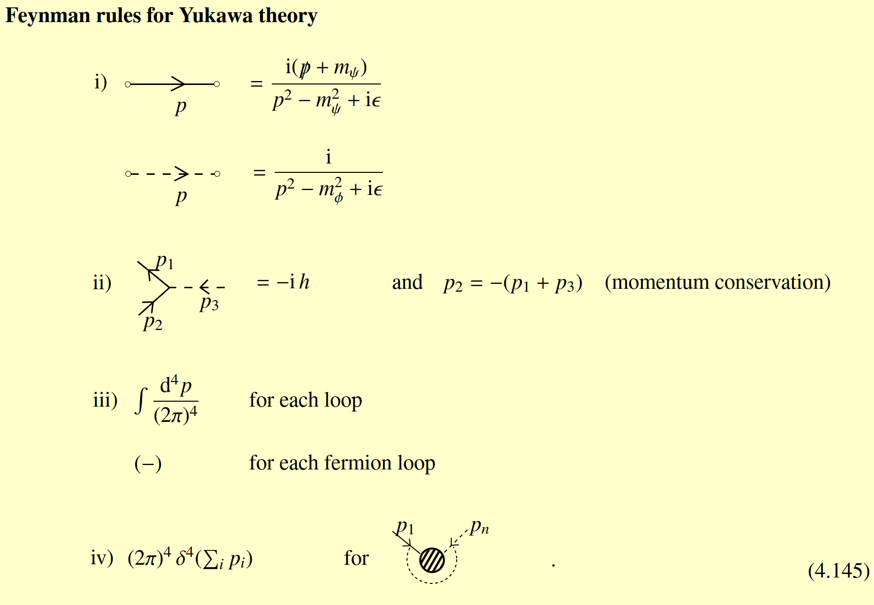
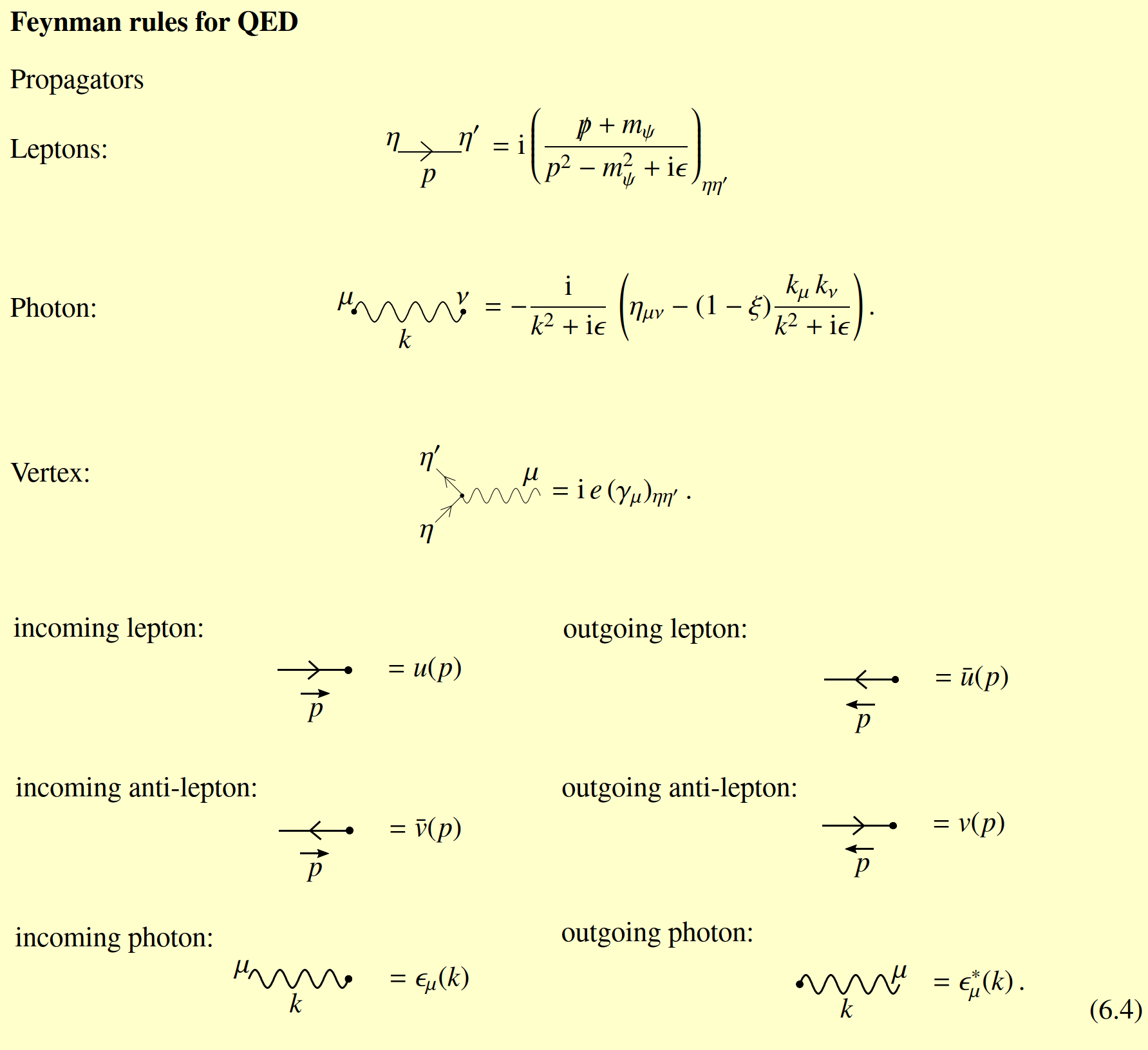
What are the Feynman rules for a Yukawa theory and for QED?↩
What is a gauge symmetry?↩
\(\psi(x) \rightarrow e^{\mathrm{i} e \alpha(x)} \psi(x)\)
\(\to\) The invariance of local rotation
How do fields transform under a gauge symmetry?↩
\(\phi(x) \rightarrow e^{\mathrm{i} e \alpha(x)} \phi(x) \quad A_\mu \rightarrow A_\mu+\partial_\mu \alpha\)
How do \(\phi_0\), \(Z\), \(\phi\) scale under \(\mu\) and \(\Lambda\)?↩
Re-parameterize \(\phi_0=Z_\phi^{1 / 2} \phi\)
We fix \(Z\) to a certain momentum scale \(p^2=\mu^2\)
we have \(\mu \frac{d\{\text{Phy. Ob}\}}{d \mu} =0\)
\(\Lambda\) is the cutoff scale with the propagator wick rotated.
General scheme:
- IR from massless particles
- UV from interaction loops \(\int \frac{d^4 \kappa}{\kappa^{2 n_b+2 n_f^{+I}}}\), but converge when no IA
Procedure:
- Perturbation at \(\phi\)
- Re-parameterize \(g,m,\phi\)
- Feynman rules, add counter term and remove the divergence
- Two method
- \(\Lambda\) cutoff and get renormalization condition
- \(\begin{array}{r}{[\langle T \phi \phi\rangle(p)]_{p^2=m^2}^{-1}=0} \\ \mathrm{i} \frac{\partial}{\partial p^2}[\langle T \phi \phi\rangle(p)]_{p^2=m^2}^{-1}=1\end{array}\)
- \(\left.\prod_i\left[\langle T \phi \phi\rangle\left(p_i\right)\right]^{-1} \cdot\left\langle T \phi\left(p_1\right) \cdots \phi\left(p_4\right)\right\rangle\right|_{s=t=u=m^2}=-\mathrm{i} \lambda\)
- Dimensional regularization at \(d=4−2\epsilon\) and remove the parameter \(\mu\) to get renormalization group equation.